Since determination of geographical origin is generally difficult based on genetic information and other bioinformation possessed innately by agricultural products, information on acquired substances in agricultural products is used. In this type of determination, techniques based on information of elements introduced in agricultural products from external sources have excellent stability and have been used in research for many years.
In addition to substances introduced from external sources, the acquired substances in agricultural products also include substances that are produced internally, such as amino acids, organic acids, fatty acids, and sugars. These substances, called metabolites as a general term, are contained in common in many agricultural products, and their concentration is thought to change dynamically at a timing determined by the surrounding environment, even in the same type of agricultural product. Therefore, if it is possible to discover patterns in the abundance ratio of the metabolites in a designated type of agricultural product in various geographic regions by comprehensive measurement of the metabolites in that agricultural product, it should be possible to use those patterns to determine the geographical origin of products produced in different regions.
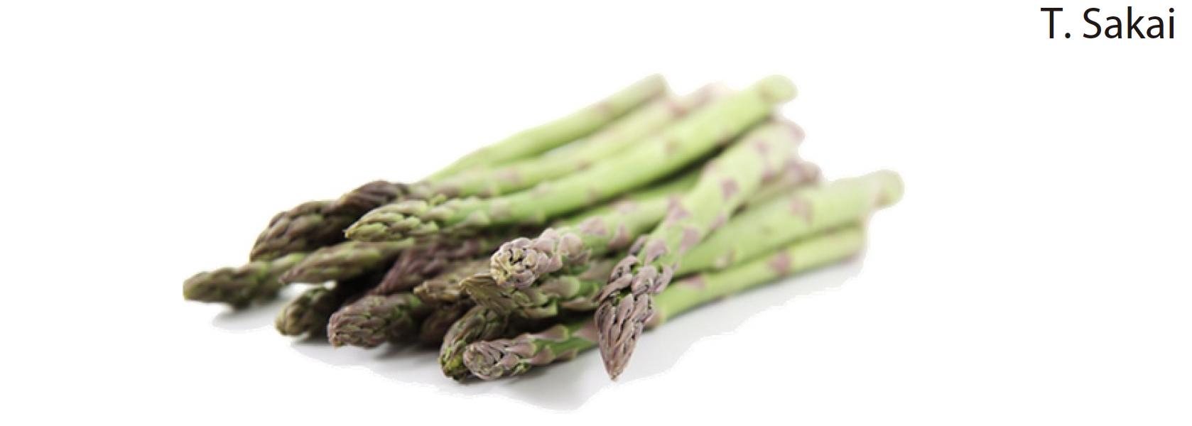
In this article, the metabolites in a total of 106 samples of domestic Japanese asparagus and asparagus produced in other countries were measured using Shimadzu Smart Metabolites Database, which enables simultaneous measurement of the compositions of 337 hydrophilic metabolites, and a model for determination of domestic or foreign origin was prepared. The results of this experiment confirmed that determination with accuracy of approximately 90% is possible.
FTIR spectroscopy is suitable to determine the relative amount of different secondary structure of proteins. This information can be obtained from the amide band I of protein in the IR spectrum, ranging from 1600 cm-1 to 1700 cm-1. Mathematical procedures such as band curve-fitting and second derivatives can be applied to resolve the overlapping amide I band components and quantify the secondary structure of proteins. In this application news, the secondary structure of mAbs is examined by using FTIR spectroscopy and band curve-fitting data analysis.
Extraction and Derivatization of Metabolites from Asparagus
The asparagus samples prepared for this experiment comprised 58 domestic Japanese samples and 48 samples of foreign origin. Asparagus, which had been cut to a suitable size, was reduced and freeze-dried, after which the samples were powdered. The obtained powders were then extracted and derivatized by a pretreatment protocol based on the Bligh & Dyer method. For details concerning the Bligh & Dyer method, please refer to Shimadzu catalog “Pretreatment Procedure Handbook for Metabolites Analysis” (C146-2181).
The internal standard used here was Ribitol.
Measurement of Derivatized Hydrophilic Metabolites
After derivatization, the sample solutions were measured by GCMS/ MS. The analytical conditions conformed to those in Shimadzu Smart Metabolites Database. Table 1 shows the detailed conditions.
Table 1 Measurement Conditions
GC-MS: GCMS-TQ™8040 NX
Column: BPX-5 (30 m × 0.25 mm, 0.25 μm)
-GC-
Injection Mode: Split (30 : 1)
Vaporizing Chamber Temperature: 250 °C
Column Oven Temperature: 60 °C (2 min) → (15 °C/min) → 330 °C (3 min)
Control Mode: Linear Velocity (39.0 cm/s)
Purge Flow Rate: 5.0 mL/min
-MS-
Measurement Mode: MRM
Ion Source Temperature: 200 °C
Interface Temperature: 280 °C
Event Time: 0.25 s
Detection of Peaks
Peak detection work was done using Shimadzu’s analysis software LabSolutions Insight™ (ver. 3.5). The following rules were set for peak detection.
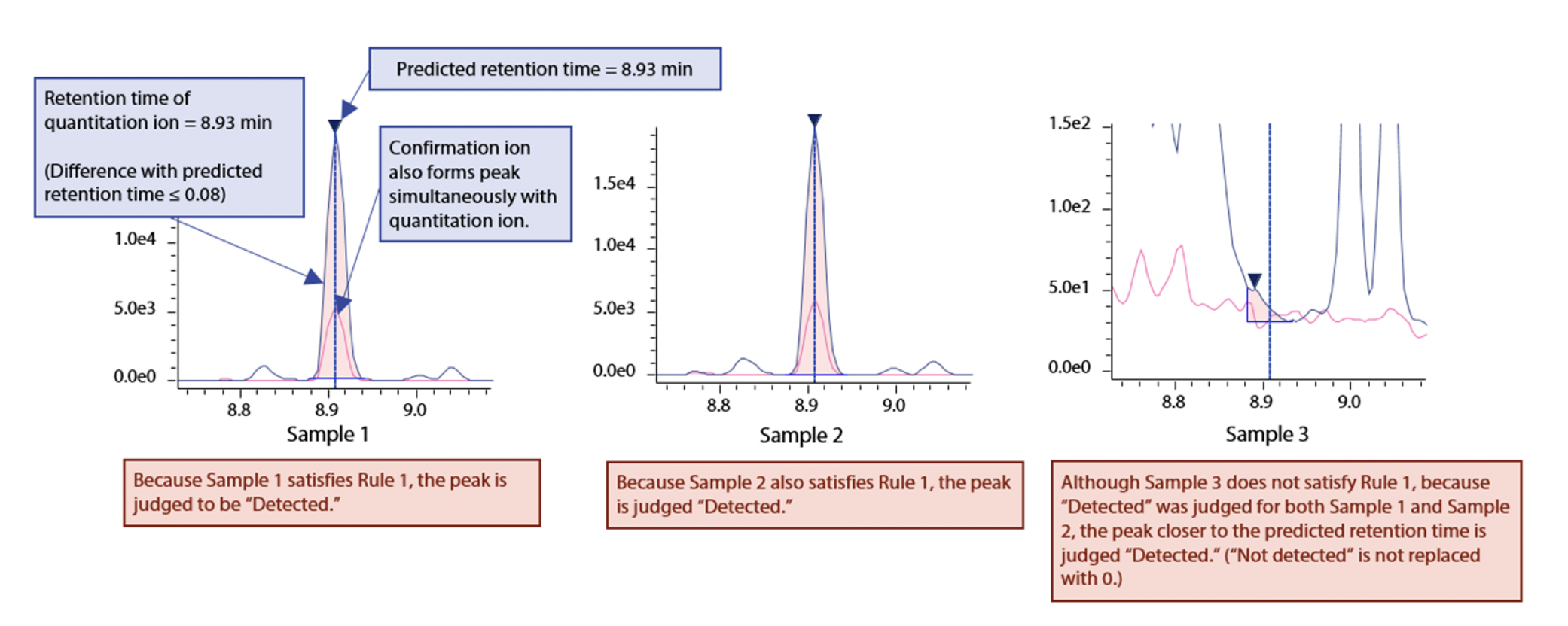
Rule 1:
Compounds for which the quantitation transition and the confirmation transition form peaks simultaneously within the retention time of ±0.08 min predicted from the retention index, and the height of the quantitation ion is also 1,000 or more, are judged to be “Detected” (Fig. 1).
Rule 2:
Even in case several of the data do not satisfy Rule 1, compounds that are judged to be “Detected” in at least half of the data are considered to be “Detected” if they resemble a peak close to the predicted retention time (in order to avoid cases where “Undetected” data become a missing value or zero: see Fig. 1).
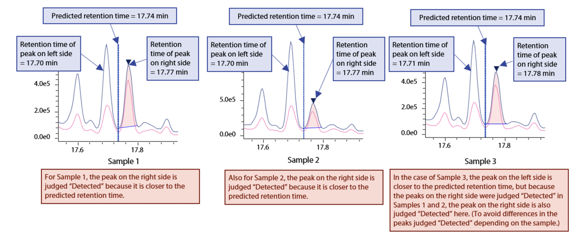
Rule 3:
In case there are 2 or more peaks that should be judged “Detected” near the predicted retention time, basically, the closer peak is considered “Detected,” but if this differs depending on the sample, the peak that was judged “Detected” in at least half of the samples is considered “Detected” (in order to avoid cases where peaks that differ depending on the sample are considered “Detected”: see Fig. 2).
Because LabSolutions Insight has the optimum functions for this type of peak detection work, detection work is possible in a short time, even in analyses that require a large number of data, such as machine learning. In this experiment, many peaks with stable shapes were obtained by GC-MS/MS measurement, enabling detection of a large number of peaks (total of 217 components).
Creation of Model for Determination of Geographical Origin
After peak detection work, the heights of all peaks were output as a data matrix, and data pretreatment was done in the same manner as described in Application News No. M282. Treatment of missing values was omitted because no data rows containing missing values existed as a result of peak detection based on the above-mentioned rules. Samples in which the peak of the internal standard was no more than the standard value were regarded as anomalies caused by the derivatization process and were deleted from the data matrix. For all other samples, the values obtained by dividing the respective peak area values by the peak area value of the internal solution were normalized by the z-score and used as data.
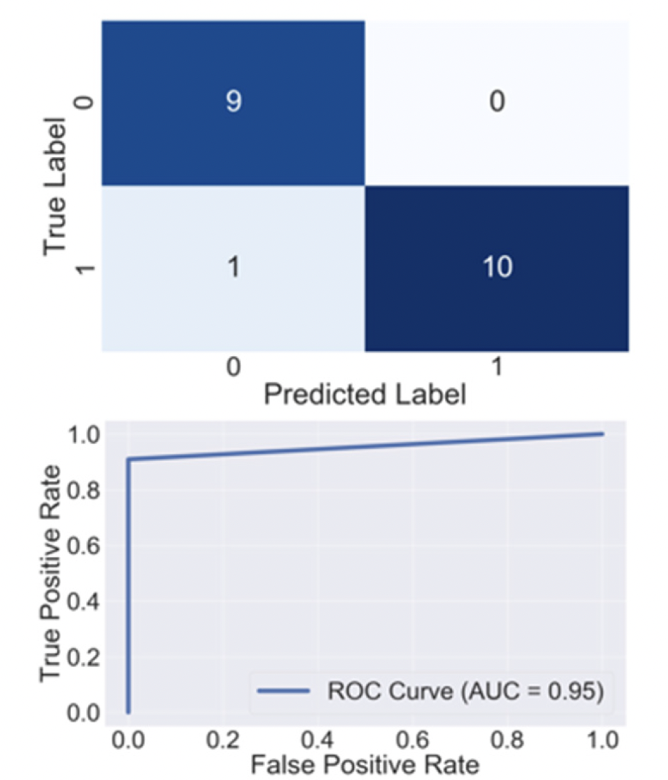
As in Application News No. M282, after randomly dividing all samples into a training set and a test set, we checked the boxplots and distributions of outliers of the 217 components for which peaks were detected, and selected 13 components that appeared to be effective for determination. A model for determination of geographical origin was then created with those 13 components using a Random Forest algorithm. An operation in which the training set and test set in the samples were randomly replaced was carried out 50 times. When predictive accuracy was calculated by applying each of the models generated in this process, the average model accuracy was 91.7%. Fig. 3 shows a representative Confusion Matrix and ROC curve obtained by this model.
This experiment suggested the possibility that comprehensive measurement of hydrophilic metabolites can be applied to determination of the geographical origin of agricultural products.